Kalman filter example

Introduction

The Kalman filter is a very useful mathematical tool for merging multi-sensor data. We’ll consider a very simple example for understanding how the filter works. Let’s consider a robot that move in a single direction in front of a wall. Assume that the robot is equipped with two sensors : a speed measurement sensor and a distance measurement sensor (range finder). We’ll consider in the following that both sensors are noisy.

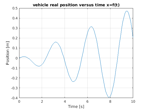
Our goal is to estimate, as accurately as possible, the position x of the robot:

Input of the system are a noisy distance measurement and a noisy velocity measurement:

Results

The results show that merging data from both sensors highly reduce incertainty (red lines) and global estimation is quite close from real position:

Source code

close all;
clear all;
clc;

% Step time
dt=0.1;
% Variance of the range finder
SensorStd=0.03;
% Variance of the speed measurement
SpeedStd=0.2;

%% Compute the vehicle trajectory and simulate sensors
% Time
t=[0:dt:10];
n=size(t,2)
% Trajectory
x=0.05*t.*cos(2*t);
% Speedometer
u=[0,diff(x)/dt] + SpeedStd*randn(1,n);
% Range finder
z=x-SensorStd*randn(1,n);

% Display position
figure;
plot (t,x);
grid on;
xlabel ('Time [s]');
ylabel ('Position [m]');
title ('Vehicle real position versus time x=f(t)');

% Display velocity
figure;
plot (t,u,'m');
grid on;
hold on;
plot (t,[0,diff(x)/dt]+3*SpeedStd,'k-.');
plot (t,[0,diff(x)/dt]-3*SpeedStd,'k-.');
xlabel ('Time [s]');
ylabel ('Velocity [m/s]');
title ('Velocity versus time u=f(t)');

% Display range finder
figure;
plot (t,z,'r');
grid on;
hold on;
plot (t,x+3*SensorStd,'k-.');
plot (t,x-3*SensorStd,'k-.');
xlabel ('Time [s]');
ylabel ('Distance [m]');
title ('Distance versus time z=f(t)');

%% Kalman

B=dt;
F=1;
Q=(SpeedStd*dt)^2;
H=1;
R=SensorStd^2;

x_hat=[0];
y_hat=[0];
P=[0];
S=[0];

for i=2:n

    %% Prediction

    %State
    x_hat(i)=F*x_hat(i-1) + B*u(i-1);

    % State uncertainty
    P(i)=F*P(i-1)*F' + Q;

    %% Update    

    % Innovation or measurement residual
    y_hat(i) = z(i)-H*x_hat(i);

    % Innovation (or residual) covariance
    S = H*P(i)*H'+R;

    K = P(i)*H'* inv(S);

    x_hat(i) = x_hat(i) + K*y_hat(i);

    P(i) = (1-K*H)*P(i);    
end

figure;
plot (t,x,'k');
hold on;
plot (t,x_hat);
plot (t,x_hat+sqrt(P),'r-.');
plot (t,x_hat-sqrt(P),'r-.');
legend('Real position','Estimated position','Uncertainty');

grid on;
xlabel ('Time [s]');
ylabel ('Distance [m]');
title ('Estimated position');

Download

This example has been inspired by the very good tutorial of Bradley Hiebert-Treuer “An Introduction to Robot SLAM (Simultaneous Localization And Mapping)”

introduction-to-slam.pdf

---