Least square approximation with a second degree polynomial

Hypotheses

Let's assume we want to approximate a point cloud with a second degree polynomial: $ y(x)=ax^2+bx+c $.

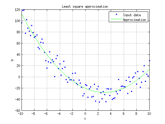
The point cloud is given by $n$ points with coordinates $ {x_i,y_i} $. The aim is to estimate $ \hat{a} $, $ \hat{b} $ and $ \hat{c} $ where $ y(x)=\hat{a}x^2+\hat{b}x + \hat{c} $ will fit the point cloud as mush as possible. We want to minimize for each point $ x_i $ the difference between $ y_i $ and $ y(x_i) $, ie. we want to minimize $ \sum \limits_{i=1}^n{(y_i-y(x_i))^2} $.

The matrix system

The matrix form of the system is given by:

$$ \left[ \begin{matrix} {x_1}^2 & x_1 & 1 \\ {x_2}^2 & x_2 & 1 \\ ... & ... & ... \\ {x_n}^2 & x_n & 1 \\ \end{matrix} \right]. \left[ \begin{matrix} \hat{a} \\ \hat{b} \\ \hat{c} \end{matrix} \right] = \left[ \begin{matrix} y_1 \\ y_2 \\ ... \\ y_n \\ \end{matrix} \right] $$

Let's define $A$, $B$ and $\hat{x}$:

$$ \begin{matrix} A=\left[ \begin{matrix} {x_1}^2 & x_1 & 1 \\ {x_2}^2 & x_2 & 1 \\ ... & ... & ... \\ {x_n}^2 & x_n & 1 \\ \end{matrix} \right] & B=\left[ \begin{matrix} y_1 \\ y_2 \\... \\ y_n \\ \end{matrix} \right] & \hat{x}=\left[ \begin{matrix} \hat{a} \\ \hat{b} \\ \hat{c} \end{matrix} \right] \end{matrix} $$

The system is now given by:

$$ A.\hat{x}=B $$

Solving the system

The optimal solution is given by:

$$ \hat{x}=A^{+}.B = A^{T}(A.A^{T})^{-1}.B $$

Where $ A^{+} $ is the pseudoinverse of $ A $. $ A^{+} $ can be computed thanks to the following formula :

$$ A^{+}=A^{T}(A.A^{T})^{-1} $$

Source code

The following Matlab source code was used for drawing the above figure:

%% Matlab script for least square linear approximation
%% This script shows the approximation with a second degree polynom
%% Written by Philippe Lucidarme
%% http://lucidar.me
close all;
clear all;
clc;

% Set the coefficients a, b and c (y=ax²+bx+c)
a=0.8;
b=-5;
c=-20;
Noise=10;

% Create a set of points with normal distribution
X=[-10:0.2:10];
Y=a*X.*X + b*X + c + Noise*randn(1,size(X,2));

% Prepare matrices
A=[ (X.*X)' ,  X' , ones(size(X,2),1) ];
B=Y';

% Least square approximation
x=pinv(A)*B;

% Display result
plot (X,Y,'.');
hold on;
plot (X,A*x,'g');
grid on;
xlabel ('x');
ylabel ('y');
legend ('Input data','Approximation');
title ('Least square approximation');Supposons que l’on veuille approximer un nuage de points avec un polynôme du second degré :

Download

Matlab source code (example on this page) can be download here: