Understanding covariance matrices

This aim of this article is to explain covariance matrices. We start from a very simple illustration (a normally uncorrelated distributed random sample) to more advanced ones (normally and correlated distribution). We finally explain how to extract usefull information from the covariance.

Uncorrelated samples

For a better understanding of the covariance matrix, we’ll first consider some simple examples. Let’s assume a gaussian distribution of random points in $ \mathbb{R}^2 $ with a standard deviation of 1 along each axis and the probability associated as illustrated on the following figure:

Figure a.

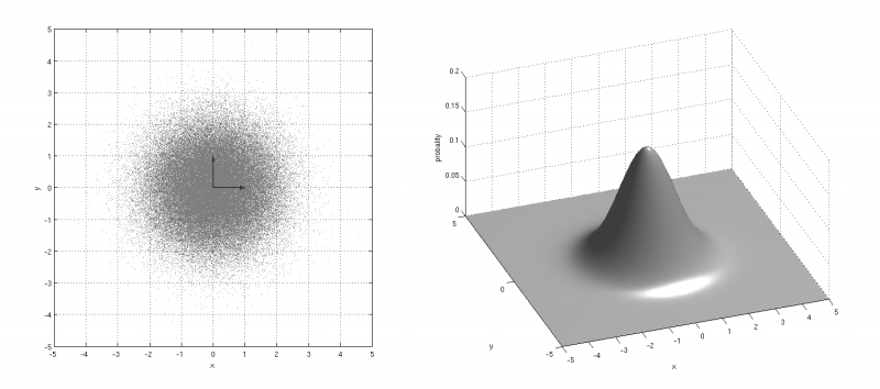As $x$ and $y$ are independant (or uncorrelated), the covariance matrix is diagonal and more precisely an identity matrix due to the standard deviations equal to 1 ( $ _a\sigma_x = {_{a}\sigma_y} = 1 $ ) in the following equation:

$$ \Sigma_a= \begin{bmatrix} _a\sigma_x^2 && 0\\ 0 && _a\sigma_y^2 \end{bmatrix} = \begin{bmatrix} 1 && 0\\ 0 && 1 \end{bmatrix} $$

On the following figure, the standard deviation along $x$ is now equal to 2 ( $ _b\sigma_x=2 $ and variance is equal to $ 2^2 $ ) with $x$ and $y$ still uncorrelated.

Figure b.

The covariance matrix is given by the following matrix:

$$ \Sigma_b= \begin{bmatrix} _b\sigma_x^2 && 0\\ 0 && _b\sigma_y^2 \end{bmatrix} = \begin{bmatrix} 4 && 0\\ 0 && 1 \end{bmatrix} $$

Note that a transformation matrix is hidden behind $\Sigma_b$. As shown on the following equation, $S_b$ is the scaling matrix that transforms the random vector from figure a into figure b.

$$ \sqrt{\Sigma_b}=S_b= \begin{bmatrix} 2 && 0\\ 0 && 1 \end{bmatrix} $$

Correlated samples

Considering now that $x$ and $y$ are linearly correlated, the sample shown on figure c. can be seen as a rotation of figure b.

Figure c.

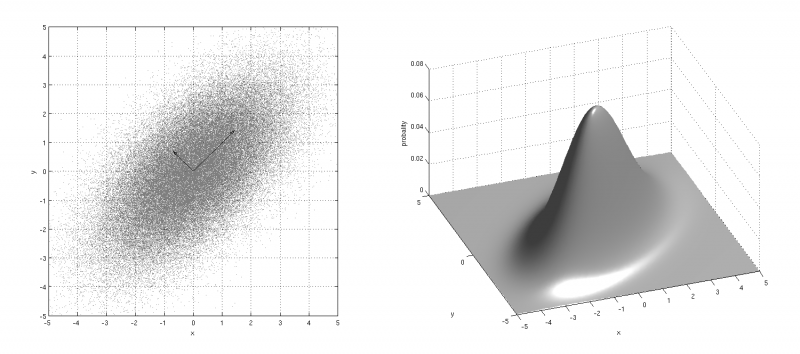The covariance matrix can be rewriten:

$$ \Sigma_c=R.\Sigma_b.R^T $$

If we assume that the angle of rotation between figure b. and c. is equal to $ \psi $, the rotation matrix $R$ is given by:

$$ R= \begin{bmatrix} cos(\psi) && -sin(\psi)\\ sin(\psi) && cos(\psi) \end{bmatrix} $$

Singular Value Decomposition (SVD)

The covariance matrix generalizes the notion of variance to multiple dimensions and can also be decomposed into transformation matrices (combination of scaling and rotating). These matrices can be extracted through a diagonalisation of the covariance matrix. In this equation the diagonal matrix $S$ is composed of the standard deviations of the projection of the random vector into a space where variables are uncorrelated:

$$ \Sigma=R.(S.S).R^T $$

where:

$R$ is a rotation matrix (eigenvectors);
$S$ is a scaling matrix (square root of eigenvalues).

The combined tranformation matrix $T_{RS}$ can easily be computed from the covariance matrix thanks to the following equation:

$$ \sqrt{\Sigma}=T_{RS}=R.S $$

The product of the transformation matrix $T_{RS}$ by the unity circle (or a N-Sphere with radius 1 in $\mathbb{R}^N$) produces an ellipse (or an ellipsoid in $ \mathbb{R}^N) $ illustrating the uncertainty. This transformation may be especially usefull. It can, for example, be used for displaying the confidence we may have in a measurement or an estimation.

Download

The figures on this page has been created with the following simple Matlab Script:

CovarianceDecomposition.m

Understanding covariance matrices

Uncorrelated samples

Correlated samples

Singular Value Decomposition (SVD)

Download

See also