Geometric model for differential wheeled mobile robot
In the following, the geometric model is a mathematical transformation where the inputs are the angular velocities of the wheels (usualy measured with encoders) and the output is the pose (position and orientation) of the mobile robot in the working space.
Problem specification
We focus here on a differential wheeled mobile robot. Such robot is composed of two wheels aligned on the same axis. Here is an illustration of Rat-Courci, a small differential wheeled robot designed for the Micromouse competition:

The wheel diameter is given by \(D=2.r\) where \(r\) is the radius. The distance between the center of the robot and the wheels is given by \(l\), the distance between wheels is \(2 \times l \) according to the following illustration:
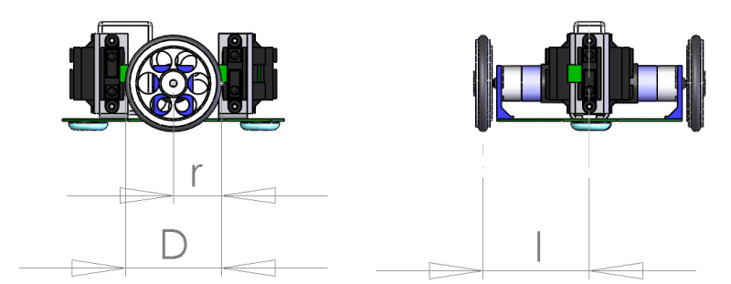
We’ll assume that the following parameters are known:
- \(r\) is the radius of the wheels;
- \(l\) the distance between the center of the robot and the wheels;
- \(\omega_l\) and \(\omega_r\) are the instantaneous angular velocities of respectively the left and right wheels.
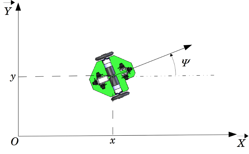
Our goal is to calculate the pose of the robot according to the upper figure:
- \(x\) and \(y\) are the coordinates of the robot
- \(\psi\) is the angular orientation of the robot
Elementary displacement calculation
First, let's calculate the linear velocity of each wheel:
$$ \begin{array}{r c l} v_l &=& r.\omega_l \\ v_r &=& r.\omega_r \end{array} $$
The average velocity of the robot is then given by:
$$ v_{robot}=\frac {v_l + v_r} {2} $$
The robot velocity can now be projected along the \(x\) and \(y\) axes:
$$ \begin{array}{r c l} \Delta_x &=& v_{robot}.cos(\psi) &=& \frac {r}{2} [ \omega_l.cos(\psi) &+& \omega_r.cos(\psi) ] \\ \Delta_y &=& v_{robot}.sin(\psi) &=& \frac {r}{2} [ \omega_l.sin(\psi) &+& \omega_r.sin(\psi) ] \end{array} $$
The angular velocity of the robot is given by the difference of the wheels linear velocities:
$$ 2.l.\Delta_{\Psi}=r.\omega_r - r.\omega_l$$
Previous equation can be reformulated as:
$$ \Delta_{\Psi}=\frac {r.\omega_r - r.\omega_l} {2.l} $$
The elementary displacement of the robot is given by the following relation:
$$ \left[ \begin{matrix} \Delta_x \\ \Delta_y \\ \Delta_{\Psi} \end{matrix} \right]= \frac{r}{2} \times \left[ \begin{matrix} cos(\psi) & cos(\psi) \\ sin(\psi) & sin(\psi) \\ \frac{1}{l} & \frac{-1}{l} \end{matrix} \right] \times \left[ \begin{matrix} \omega_r \\ \omega_l\end{matrix} \right] $$
Absolute position
The absolute position can be calculated thanks to the following equations:
$$ \begin{array}{r c l} x_{i}&=&x_{i-1}+\Delta_x \\ y_{i}&=&y_{i-1}+\Delta_y \\ \Psi_{i}&=&\Psi_{i-1}+\Delta_{\Psi} \end{array} $$
where
- \(x_{i}\) and \(y_{i}\) are the coordinates of the robot at time step \(i\);
- \(\Psi_{i}\) is the orientation of the robot at time step \(i\).
Of course, this model has some limitations. The result is highly dependant on the accuracy of the robot (mechanical assembly, wheel diameter, distances ...). We assume that wheels rotate without any slippery problems which is not true in practice. We also assume that the sampling rate is fast enough to assume that \(\Delta_x\), \(\Delta_y\) and \(\Delta_\Psi\) will remain elementary displacements.
See also
- Angular and linear velocity, cross product
- Configurable gear for solidwork
- Elastic collision - Part 1 - Hypotheses
- Elastic collision - Part 2 - Velocity decomposition
- Elastic collision - Part 3 - Velocity calculation
- Elastic collision - Part 4 - Synthesis and reminder
- Elastic collision - Part 5 - Source code
- Elastic collision - Equations and simulation
- Enable Add-Ins in Solidworks
- Newton's Second Law of motion
- How to insert gears in a Solidwoks assembly
- Mathematical model of a mechanical differential
- Model of a rotary joint driven by a linear motor [Part 2]
- Model of a rotary joint driven by a linear motor [Part 3]
- Model of a rotary joint driven by a linear motor [Part 4]
- Model of a rotary joint driven by a linear motor